5 Testing alternative hypotheses

In this section we focus on specific alternative hypotheses for diversification rates. The first part of our congruence class exploration focuses on specific alternative models. That is, we first start by providing a set of alternative extinction rate functions and compute the matching speciation rate functions. Then, we turn the approach around and specify some alternative speciation rate functions for which we compute the matching extinction rate functions.

5.1 Testing alternative extinction rates

In this subsection we focus entirely on alternative hypotheses of extinction rates for which we compute the resulting speciation rates.

5.1.1 Constant extinction rates

Let us assume that the extinction rate was constant, but at a range of different values. Specifically, let’s assume that the true extinction rate was \(\mu(t)=\{0.0,0.025,0.05,0.075,0.1\}\). For our models we need to create extinction rate functions with these values.

mu_vals <- seq(0,0.1,0.025)
mu1 <- list()
for (i in 1:length(mu_vals)) {
  mu1[[i]] = local({
    mu = mu_vals[i]
    function(t) { rep(mu,length(t)) }
  })
}

Now we compute the new speciation rate given the extinction rates.

alt_models <- congruent.models(my_model, mus = mu1)

Let’s have a look at these alternative models.

plot( alt_models )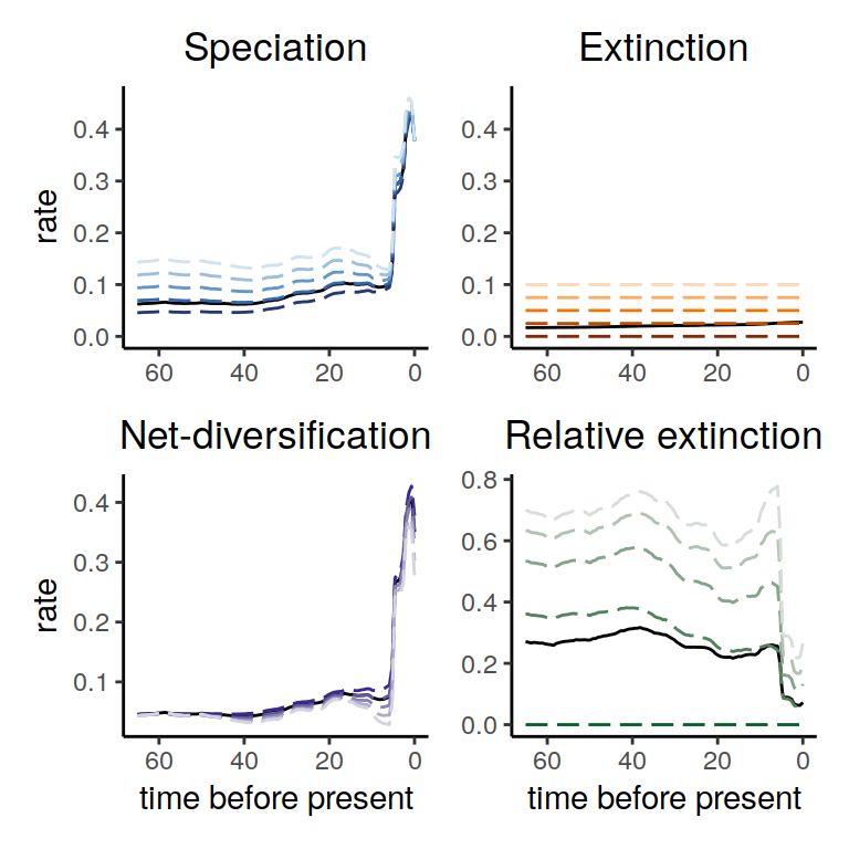

Figure 5.1: Diversification rate functions within the congruence class assuming different constant extinction rate functions. The dashed lines show the different alternatives that we explored here, and the solid lines represent our reference model. Here we notice that the overall pattern of speciation rates as well as net-diversification rates is fairly robust to alternative constant extinction rates within the congruence class. Only the relative extinction rate changes is value, which is not surprising since we explored different extinction rates.

Next, we can inspect the summary of the trends in the speciation rate through time

p <- summarize.trends(alt_models, threshold = 0.02)
plot(p)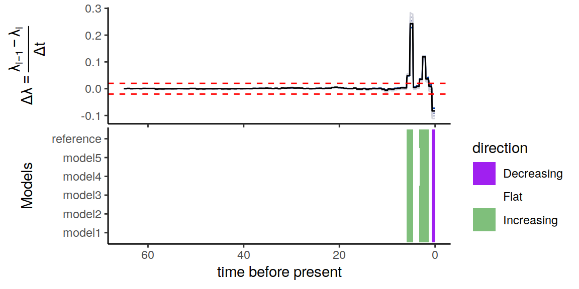

Figure 5.2: Summary of directional trends in the congruence class.

Notice that there is variation in the slope of the speciation rate (\(\Delta\lambda\)) throughout the entire time span of the phylogenetic tree. Yet, when we only consider rate changes that are smaller or greater than our threshold of \(\epsilon = 0.02 \Delta\lambda\) per million years, it becomes evident that the constructed congruent models are in complete agreement of the two increases in speciation rate, as well as the more recent decline in speciation rate.

5.1.2 Linearly increasing extinction rates

Next, we will explore different linear rate functions for the extinction rate. Let us assume that the extinction rate was linear with a range of different slopes. Specifically, let’s assume that the slope was \(\alpha=\{0.0,0.0005, \ldots, 0.002\}\). We played around with these \(\alpha\) values to get reasonable rate functions. You will need to modify these for your dataset. Note that in CRABS, rate functions are defined in backwards time, so while these look like decreasing extinction rates, they are in fact increasing extinction rates when you consider time forward from past to present.

We create extinction rate functions with these \(\alpha\) values.

mu_min = 0.01
mu_vals <- seq(0,0.002,0.0005)
mu1 <- list()
for (i in 1:length(mu_vals)) {
  mu1[[i]] = local({
    mu_slope = mu_vals[i]
    function(t) { mu_min + mu_slope * (max_t-t) }
  })
}

Now we compute the new speciation rate given the extinction rates.

alt_models <- congruent.models(my_model, mus = mu1)

Let’s have a look at these alternative models.

plot(alt_models)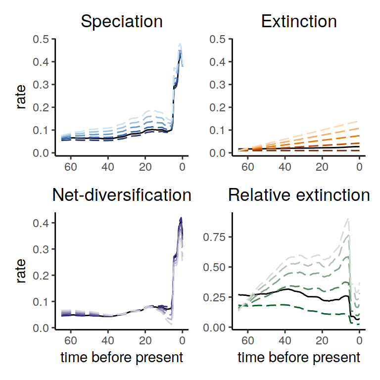

Figure 5.3: Diversification rate function for different linear extinction rates within the same congruence class. The dashed lines show the different alternatives that we explored here, and the solid lines represent our reference model. We observe that the speciation and net-diversification rates are robust to different linear extinction rates within the congruence. As expected, the relative extinction rate changes because we chose different extinction rates.

Next, we can inspect the summary of the trends in the speciation rate through time

p <- summarize.trends(alt_models, threshold = 0.02)
plot(p)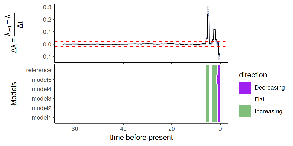

Figure 5.4: Summary of directional trends in the congruence class.

Similar to the example with constant alternative extinctionrate models, there is some variation in the trends, but the same conclusion remains. Namely, for our threshold of \(\epsilon = 0.02 \Delta\lambda\) per million years, it is evident that the constructed congruent models are in complete agreement of the two increases in speciation rate, as well as the more recent decline in speciation rate.

5.1.3 Exponential increasing extinction rates

Next, similar to the linear rate functions we explore some exponential rate functions. We start here with the exponentially increasing rates. Recall that the extinction rate is a function of time such that \(\mu(0)\) is the rate at the present and \(\mu(1)\) is the rate 1 time unit previously, thus what appear to be exponential increases are in fact decreases. Specifically, let’s assume that the growth rate was \(\alpha=\{0.0,0.005, \ldots, 0.02\}\). Then, we define the extinction rate function as

mu_max = 0.015
mu_vals <- seq(0,0.02,0.005)
mu1 <- list()
for (i in 1:length(mu_vals)) {
  mu1[[i]] = local({
    mu_factor = mu_vals[i]
    function(t) { mu_max * exp(mu_factor*(max_t-t)) }
  })
}

Now we compute the new speciation rate given the extinction rates.

alt_models <- congruent.models( my_model, mus = mu1 )

Let’s have a look at these alternative models.

plot( alt_models )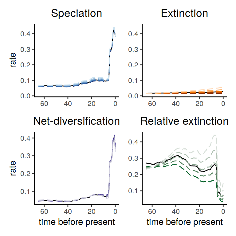

Figure 5.5: Diversification rate functions for exponentially increasing extinction rates within the congruence class. The dashed lines show the different alternatives that we explored here, and the solid lines represent our reference model. As in our previous example, the speciation rate and net-diversification rate are robust to the difference choices of extinction rates

Next, we can inspect the summary of the trends in the speciation rate through time

p <- summarize.trends(alt_models, threshold = 0.02)
plot(p)

Figure 5.6: Summary of directional trends in the congruence class.

Similar to the two previous examples, there is some variation in the trends, but the same conclusion remains. Namely, for our threshold of \(\epsilon = 0.02 \Delta\lambda\) per million years, it is evident that the constructed congruent models are in complete agreement of the two increases in speciation rate, as well as the more recent decline in speciation rate.

5.1.4 Two-epoch extinction rates

Let us assume that the extinction rate changed abruptly at a pre-defined change-point. We’ll try to fix the change-point to the estimated rapid increase in diversification. Thus, we are modeling the extinction rate as a 2-epoch model. Furthermore, let us try a range of different factors of increase/decrease. Specifically, let’s assume that the rate increase/decrease was by a factor of \(\alpha=\{1,2,4\}\). Again, we create the list of extinction rate functions.

mu_min = 0.05
t_shift = 5.5
alpha_vals <- seq(-2,2,1)
mu1 <- list()
for (i in 1:length(alpha_vals)) {
  mu1[[i]] = local({
    alpha = alpha_vals[i]
    function(t) { ifelse( t < t_shift, mu_min*2^alpha, mu_min) }
  })
}

Now we compute the new speciation rate given the extinction rates.

alt_models <- congruent.models( my_model, mus = mu1 )

Let’s have a look at these alternative models.

plot( alt_models )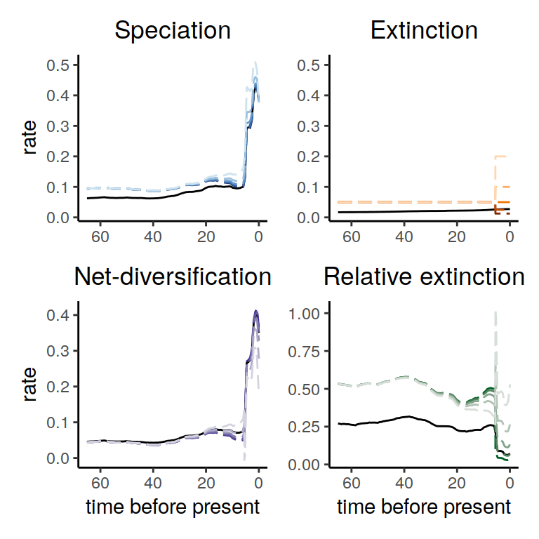

Figure 5.7: Diversification rate functions for 2-epoch extinction rate functions within the congruence class. The solid line shows the reference model and the dashed lines show the alternative models. We observe no noticeable effect on the overall trend of the derived speciation rates.

Next, we can inspect the summary of the trends in the speciation rate through time

p <- summarize.trends(alt_models, threshold = 0.02)
plot(p)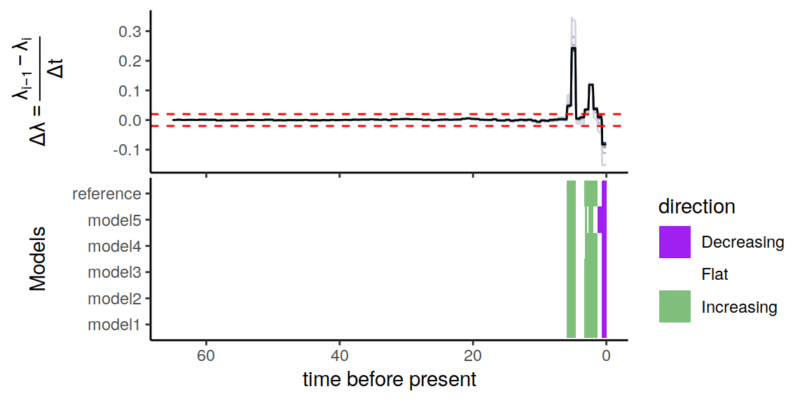

Figure 5.8: Summary of directional trends in the congruence class.

Again, for our threshold of \(\epsilon = 0.02 \Delta\lambda\) per million years, it is evident that the constructed congruent models are in complete agreement of the two increases in speciation rate, as well as the more recent decline in speciation rate.

5.1.5 Reversed trend extinction rates

As a last example, let us explore the case where the extinction rate had the opposite trend to the estimated speciation rate. That is, if the speciation rate was going up, now we model that the extinction rate goes down. This should produce the same pattern in the net-diversification rate. We create this reversed/opposite trend extinction rate function by subtracting the observed speciation rate from some arbitrary baseline (which is necessary to make sure that all extinction rates are positive).

mu_scaling <- c(1.1, 1.2, 1.5, 2.0)
mu_0s <- max(lambda(my_model$times)) * mu_scaling

mu_prime <- list()
for (i in seq_along(mu_scaling)){
  mu_prime[[i]] <- local({
    mu_0 <- mu_0s[i]
    function(t) mu_0 - lambda(t)
  })
}

Now we compute the new speciation rate given the extinction rates.

alt_models <- congruent.models(my_model, mus = mu_prime)

Let’s have a look at these alternative models.

plot( alt_models )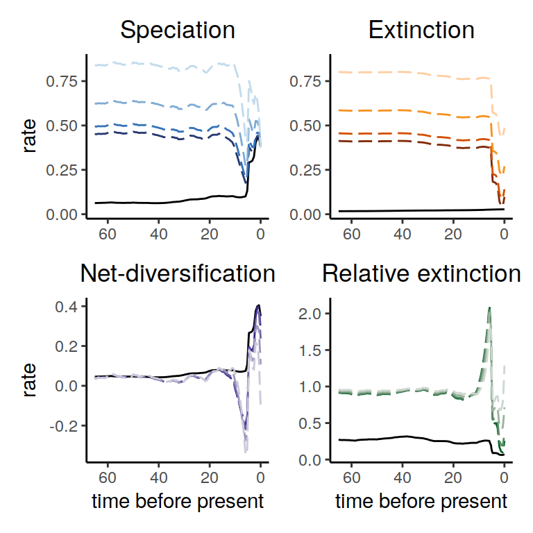

Figure 5.9: Diversification rate functions for our reversed trend additive extinction rate function. The solid line shows the reference model and the dashed lines show the alternative model. Interestingly, the reversed model where the extinction rate goes down instead of the speciation rate going up is not exactly in the congruence class, as we see that the net-diversification rates are not identical. Instead, we see that the speciation rate now drops first just to still increase towards the present.

In Figure 5.9 we used an additive trend by subtracting the rate. However, we can also use a multiplicative model by subtracting the log speciation rate and then back-transforming the extinction rate from the log-scale.

mu_min = 0.0075
mu1 <- function(t) exp(log(mu_min) - log(my_model$lambda(t)))

Now we compute the new speciation rate given the extinction rates.

alt_models <- congruent.models( my_model, mus = mu1 )

Let’s have a look at these alternative models.

plot( alt_models )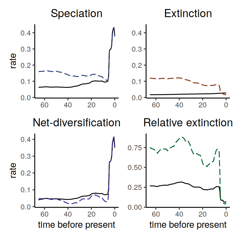

Figure 5.10: Diversification rate functions for our reversed multiplicative trend extinction rate function. The solid line shows the reference model and the dashed lines show the alternative model. Interestingly, the derived speciation rate is qualitatively identical except that the speciation rate first decreases before sharply increasing towards the present.

Since there are just two models here, it is not necessary to plot the trend summary. It is obvious that the speciation rate still exhibits a sharp increase followed by a downturn toward the present.

This concludes our brief exploration of different common shapes of extinction rates. In summary, the speciation and net-diversification rates are mostly robust to our relatively minor variations in extinction rates. Specifically, the observed pattern of a sharp increase of the speciation rate towards the present is robust to all variation of extinction rates we tested. Only if we would change the extinction rates in extreme and biologically unrealistic ways, e.g., by allowing the extinction rate to become implausible large, then the extinction rates can overwhelm our observed diversification rate pattern.

5.2 Testing alternative speciation rates

Let us now look at the congruence class from the angle of the speciation rates. Can we also specify different speciation rate function and obtain valid extinction rates?

5.2.1 Constant speciation rates

Let us assume that the speciation rate was constant. However, the congruence class as defined by Louca & Pennell (2020) dictates that \(\lambda(0) = \lambda'(0)\), assuming the same present day sampling fraction for both models. Thus, there is only one possible constant rate speciation model within the congruence class with \(\lambda'(t) = \lambda(0)\) Specifically, let’s assume that the true speciation rate was \(\lambda(t) = \lambda_0\). We follow exactly the same approach as with the extinction rates. Hence, we start by defining the speciation rate function.

lambda1 <- function(t) my_model$lambda(0.0)

Now we compute the new extinction rate given the speciation rates.

alt_models <- congruent.models( my_model, lambda = lambda1)

Let’s have a look at these alternative models.

plot( alt_models )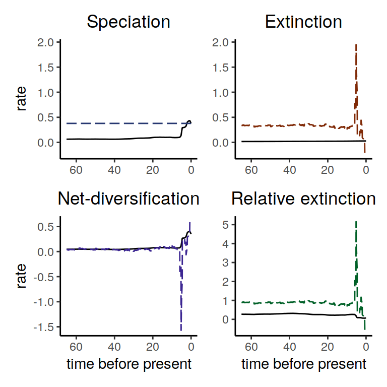

Figure 5.11: Diversification rate functions for a constant speciation rates within the congruence class. The solid line shows our reference model and the different dashed line shows the alternative model. Most interesting, we observe that for the constant speciation rate function we compute an extinction rate that was negative towards the present.

In this example we observe that for the constant speciation rate function the derived extinction rate function was negative at the near present. A negative extinction rate is clearly unrealistic. Thus, we can conclude that there is no constant rate speciation rate function within the congruence class.

5.2.2 Exponential increasing/decreasing speciation rates

Let us assume that the speciation rate was exponentially increasing or decreasing. Furthermore, let us try a range of different factors of increase/decrease. Specifically, let’s assume that the growth rate was \(\alpha=\{-0.04,-0.03,\ldots, 0.04\}\). Again, we create the list of speciation rate functions.

lambda_present = lambda(0)
alpha_vals <- c(seq(0.0,0.04,0.02),seq(-0.5,-0.1,0.2))
lambda1 <- list()
for (i in 1:length(alpha_vals)) {
  lambda1[[i]] = local({
    alpha = alpha_vals[i]
    function(t) { lambda_present * exp(alpha*t) }
  })
}

Now we compute the new extinction rate given the speciation rates.

alt_models <- congruent.models( my_model, lambda = lambda1)

Let’s have a look at these alternative models.

plot( alt_models )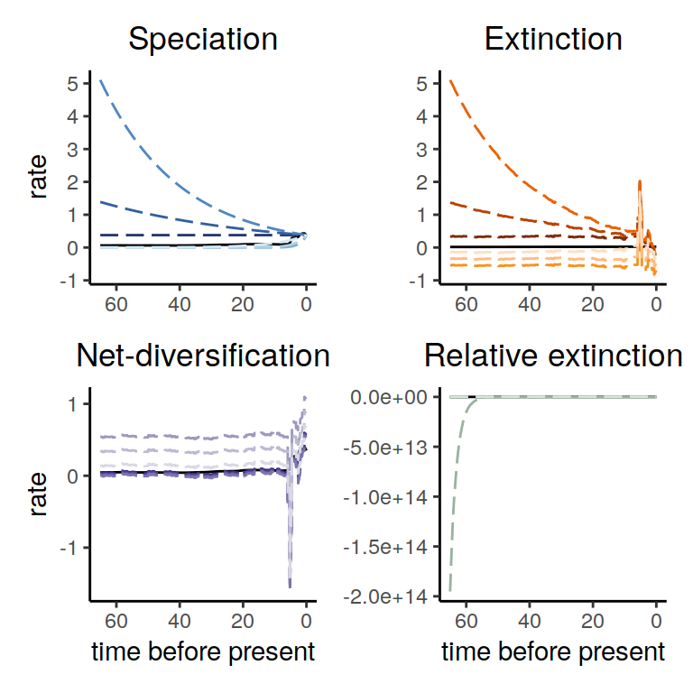

Figure 5.12: Diversification rate functions for exponentially increasing/decreasing speciation rate functions within the congruence class. The solid line shows the reference model and the dashed lines show the alternative models. Again, we observe that for all speciation rate functions that the derived extinction rate functions are negative towards the present and/or at some other point in time.

We can also plot the directional trends in the extinction rate through time:

p <- summarize.trends(alt_models, threshold = 0.02, rate_name = "mu")
plot(p)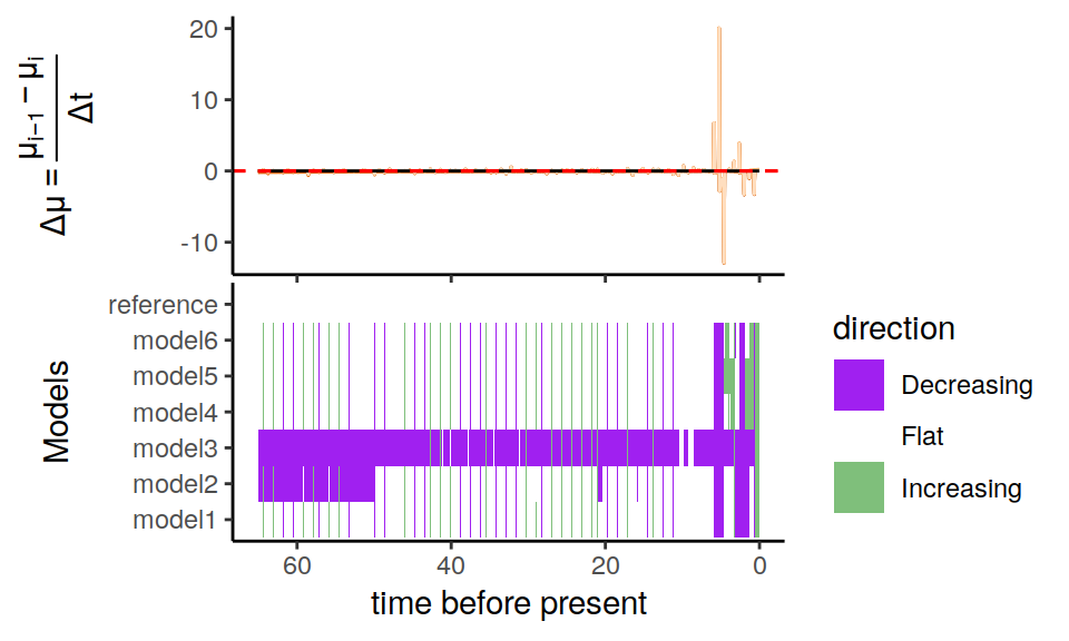

Figure 5.13: Congruence class assuming exponentially changing speciation rates.

Our results here for the exponentially increasing speciation functions show again that the derived extinction rates are negative towards the present and/or at another point in time. Because of the initial condition that all speciation rate functions within the congruence class must have the same value at time \(t=0\) (the present), it is very challenging to find other speciation rate functions that have valid extinction rates (i.e., \(\mu(t)\leq 0\)). This indicates that the congruence class is much more restrictive for the space of valid speciation rates.