4 Creating the congruence class
Here, we will start with some theoretical background (although quite simplified) on congruence class. Our main aim is to motivate, guide and explain our choices for how to explore the congruence class.
4.1 Rate transformations
One important aspect of the congruence class is that if we know the pulled rates, i.e., the pulled speciation or net-diversification rates, then we only need to know additionally either the new speciation or extinction rate to solve for the missing rate function. That means, we can compute the pulled diversification rate for our reference model, i.e., using our empirically estimated speciation and extinction rates from the previous sections, and then specify whichever alternative speciation or extinction rate function. Then we solve the pulled diversification rate equation for this new rate function.
The pulled diversification rate is defined as \[\begin{equation} r_p(t) = \lambda(t) - \mu(t) + \frac{1}{\lambda(t)} \frac{\text{d}\lambda(t)}{\text{d}t} \tag{4.1} \end{equation}\]
As you may notice, the latter part of this equation entails the derivative of the speciation rate function.
This derivative is only known for simple rate models, for example the constant rate process, linear rates or exponential rates.
For more complex models, it is often impractical or impossible to find the derivative analytically.
In order to solve (eq. ??) for \(mu(t)\), the rearrangement of \(\mu(t) = \lambda(t) - r_p(t) + \frac{1}{\lambda(t)}\frac{d\lambda}{dt}\) is trivial, and we use the finite difference method to approximate the derivative \(\frac{d\lambda}{dt}\) evaluated at time \(t\).
In order to get \(\lambda(t)\), we use an ODE (Ordinary Differential Equation) solver to compute the solution numerically. More specifically, we use a Runge-Kutta method of order five, implemented in Fortran. We use the function radau() in the R-package deSolve as an interface to access the ODE solver in R.
These are our fundamental pieces about the congruence classes. We have the reference model, from which we compute the pulled diversification rate. Then you can either specify alternative speciation or extinction rate functions, for which we then compute the matching extinction or speciation rate function respectively, or you can explore a space of speciation or extinction rate functions. We will walk through examples of these in the following sections.
4.2 Slopes and \(\Delta t\)
Given a congruence class, you may want to either visualize or summarise the models that belong to the congruence class. Visualisation of the alternative models is done in a hopefully intuitive way so we explain it later. Summarizing alternative models is somewhat less established. In our view, the main objective of these diversification functions is to estimate if speciation and/or extinction rates have changed over time. A change in rate over time is mathematically represented by the slope of the rate function; a large slope means more/steeper change in less time, while a small value for the slope corresponds to rather constant rates. Therefore, we summarize the models by computing the slope of the rate function. Then, we assess each time interval independently if the slope was larger than a specified threshold. The sign of the slope shows the direction of change, either increasing or decreasing.
We will come back to the summaries later when we created samples from the congruence class.
4.3 The model object
In order to create a congruence class, we require some information about the extinction and speciation rate functions in at least one of the models in the congruence class.
In the following examples we will use the results from an episodic birth-death model fitted in RevBayes (see Section 8.4), but we note that CRABS can work with any rate estimates.
To simplify this section, we provide the results in a convenient format:
data("primates_ebd")
head(primates_ebd)
## # A tibble: 6 × 3
## lambda mu time
## <dbl> <dbl> <dbl>
## 1 0.378 0.0274 0
## 2 0.432 0.0272 0.657
## 3 0.426 0.0271 1.31
## 4 0.402 0.0270 1.97
## 5 0.324 0.0269 2.63
## 6 0.301 0.0266 3.29We also provide an example for fitting birth-death models in TESS (Section 8.2) and TreePar (Section 8.3).
If you wish to use these results instead, simply call data("primates_ebd_treepar") or data("primates_ebd_tess").
After we have estimated our birth-death rates, we transform the data into piecewise linear rate functions in R
times <- primates_ebd[["time"]]

lambda <- approxfun(times, primates_ebd[["lambda"]])
mu <- approxfun(times, primates_ebd[["mu"]])
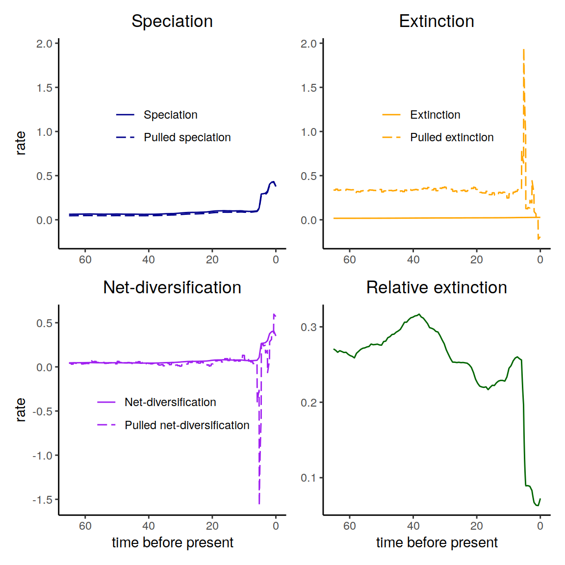
Next, we create a congruence class object which contains all the transformed rate functions (i.e., the net-diversification rate and relative extinction rate) as well as the pulled rates (i.e., the pulled net-diversification and the pulled speciation rate).
max_t <- max(primates_ebd[["time"]])
times_fine <- seq(0, max_t, length.out = 1000)

my_model <- create.model(lambda,
                         mu,
                         times_fine)
plot(my_model)
Figure 4.1: The diversification rates in the reference model.
The my_model includes all the rate functions.
You could plot these yourself, or you can use our simple plotting function.
Now that we have our reference model and congruence class functions, we can explore alternative rate functions within the congruence class.