8 Estimating birth-death models
One of the main features and aims of CRABS is to explore the congruence class for the diversification rates that you estimated using another software or R package.
Here we provide you some examples using standard software for estimating diversification rates through time, but if your preferred software is not included then you can either specify the diversification rate functions manually, or try to follow our examples in loading the output.
8.1 Reading the phylogenetic tree
First, we assume that you have a phylogenetic tree which you can load into R. There are several tutorials on how to do so (e.g., TESS or APE, and we simply refer to these tutorials here). As an example, we used the Primates phylogeny from Springer et al. (2012). You can download the data from our RevBayes tutorial. First we need to load the APE package (Paradis & Schliep, 2019).
library(ape)Now we can read our phylogenetic tree
tree <- read.tree(file="data/primates.tre")Next, read the software examples to fit birth-death models to the tree, and estimate diversification rates.
8.2 TESS Analysis
First, load the TESS package.
library(TESS)For some of our plotting, we need the speciation times. So we extract these from the tree.
btimes <- sort( as.numeric( branching.times( tree ) ) )
max_t <- max(btimes)tess.analysis(tree,
empiricalHyperPriors = TRUE,
samplingProbability = 1.0,
numExpectedRateChanges = 2,
MAX_ITERATIONS = 100000,
MAX_TIME = 2*60*60,
MIN_ESS = 625,
dir = "primates_comet")## Estimating empirical hyper-parameters.
##
## Burning-in the chain ...
## 0--------25--------50--------75--------100
## ==========================================
## Finished burnin period!
##
## Running the chain ...
## 0--------25--------50--------75--------100
## ==========================================
## Finished MCMC!
##
## Parameter | delta | Acceptance Probability
## ==========================================
## diversification | 0.152 | 0.487
## turnover | 0.031 | 0.406
##
## Performing CoMET analysis.
##
## Burning-in the chain ...
## 0--------25--------50--------75--------100
## ==========================================
##
## Running the chain ...
## 0--------25--------50--------75--------100
## ==========================================tess.output <- tess.process.output("primates_comet",
numExpectedRateChanges = 2)est_speciation <- apply(tess.output[["speciation rates"]], 2, median)
est_extinction <- apply(tess.output[["extinction rates"]], 2, median)Let us make a data frame representation of the rates. Since TESS is parameterized in forward time (i.e. with \(t = 0\) being the root of the phylogeny, increasing toward the present), we want to reverse the rates to be compatible with CRABS.
times <- seq(0, max_t, length.out = 100)

primates_ebd_tess <- tibble(
  "time" = times,
  "lambda" = rev(est_speciation),
  "mu" = rev(est_extinction),
)
head(primates_ebd_tess)
## # A tibble: 6 × 3
## time lambda mu
## <dbl> <dbl> <dbl>
## 1 0 0.194 0.337
## 2 0.721 0.592 0.337
## 3 1.44 0.593 0.355
## 4 2.16 0.592 0.421
## 5 2.88 0.586 0.477
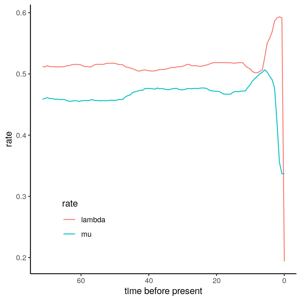
## 6 3.60 0.569 0.491Now let’s have a look at the estimated rate functions
p <- primates_ebd_tess %>%
  tidyr::gather("rate", "value", -time) %>%
  ggplot(aes(x = time, y = value, color = rate)) +
  geom_line() +
  theme_classic() +
  scale_x_reverse() +
  theme(legend.position = c(0.2, 0.2)) +
  labs(y = "rate", x = "time before present")
plot(p)
Figure 8.1: The estimated posterior median results from an episodic birth-death model fitted in RevBayes.
The data frame primates_ebd_tess is what we get when we call the data("primates_ebd_tess") function in CRABS. We use the RevBayes estimated rates in our vignette examples, but it is easy to substitute those for the TESS analysis results to construct the congruence class.
8.3 TreePar
Let us walk here through a very simple TreePar analysis (Stadler, 2011). For a real publication worthy analysis, you may want to do a more thorough analysis by allowing more possible shifts and a finer grid for the search space.
First, load the TreePar package.
library(TreePar)TreePar needs the ages of the phylogeny to perform it’s likelihood computation. We use the TreePar builtin functionality for this.
x     <- sort(getx(tree),decreasing=TRUE)
max_t <- max(x)
For our toy analysis, we setup some simpler than normal search values. We specify that there are at most three rate shifts, and that there are ten possible shift points. For your own analysis, you should most likely increase these values. We also specify an interval offset of 0.05, which means that in the most recent 5% of the tree age there was no rate shift event. This is simply for improving the parameter estimation.
MAX.NUM.SHIFTS  = 4
NUM.INTERVALS   = 20
INTERVAL.OFFSET = 0.05
Now we run the full TreePar maximum likelihood search.
res   <- bd.shifts.optim(x,
                         sampling=rep(1,MAX.NUM.SHIFTS+1),
                         grid=max_t/NUM.INTERVALS,
                         start=INTERVAL.OFFSET*max_t,
                         end=max_t,
                         survival=1,
                         posdiv=TRUE)[[2]]
Now we have the maximum likelihood estimates for the different number of shifts. We want to test if \(i\) shifts explain the tree significantly better than \(i-1\) shifts.
best <- 0
for (i in 1:(length(res)-1)) {
    test <- pchisq(2*(res[[i]][1]-res[[i+1]][1]),3)
    #if test>0.95 then i shifts is significantly
    # better than i-1 shifts at a 5% error
    if ( test > 0.95 ) {
        best <- i
    } else {
        break
    }
}
best_result <- res[[best+1]]
speciation <- c()
extinction <- c()
for (i in 1:(best+1)) {
speciation[i] <- best_result[1+i+(best+1)] /
(1-best_result[1+i])
extinction[i] <- best_result[1+i+(best+1)] /
(1/best_result[1+i]-1)
}
if ( best > 0 ) {
shift_times <- best_result[ (length(best_result)-best+1) :
length(best_result)]
tmp_lambda <- function(x) {
index <- findInterval(x, shift_times);
return ( speciation[index+1] )
}
tmp_mu <- function(x) {
index <- findInterval(x, shift_times);
return ( extinction[index+1] )
}
lambda <- Vectorize(tmp_lambda)
mu <- Vectorize(tmp_mu)
} else {
lambda <- function(x) { return ( rep(speciation[1],length(x)) ) }
mu <- function(x) { return ( rep(extinction[1],length(x)) ) }
}Let us make a data frame representation of the rate functions
times <- seq(0, max_t, length.out = 100)

primates_ebd_treepar <- tibble(
  "time" = times,
  "lambda" = lambda(times),
  "mu" = mu(times),
)
head(primates_ebd_treepar)
## # A tibble: 6 × 3
## time lambda mu
## <dbl> <dbl> <dbl>
## 1 0 0.392 0.00000181
## 2 0.721 0.392 0.00000181
## 3 1.44 0.392 0.00000181
## 4 2.16 0.392 0.00000181
## 5 2.88 0.392 0.00000181
## 6 3.60 0.243 0.216Now let’s have a look at the estimated rate functions
The data frame primates_ebd_treepar is what we get when we call the data("primates_ebd_treepar") function in ACDC. We use the RevBayes estimated rates in our vignette examples, but it is easy to substitute those for the two-epoch TreePar results to construct the congruence class.
8.4 The HSMRF model in RevBayes
RevBayes (Höhna et al., 2016) provides several methods to estimate diversification rates through time.
Here we used the https://revbayes.github.io/tutorials/divrate/ebd.html using the episodic-birth-death model with a Horseshoe-Markov-Random-Field (HSMRF) prior distribution to estimate diversification rates (Magee et al., 2020).
We assume here that you followed the RevBayes tutorial and have the output stored as a log-file in the output folder.
If you have not run a RevBayes analysis and wish to explore functionality of the package, we have provided a thinned output file, accessible with data("primates_ebd_log").
For some of our plotting, we need the speciation times. So we extract these from the tree.
btimes <- sort( as.numeric( branching.times( tree ) ) )
max_t <- max(btimes)
Then we read in the RevBayes log-file as a simple tab-delimited file.
#samples <- read.table(file="output/HSMRFBDP_primates.log",
#                      stringsAsFactors=FALSE,
#                      header=TRUE)
data("primates_ebd_log")
samples <- primates_ebd_log
Then, from this log-file we want to automatically extract the speciation and extinction rates. Be careful that you used the same names as we did. Otherwise you need to modify this code-snippet accordingly.
par_speciation <- samples[, startsWith(names(samples), "speciation_rate.")]
par_extinction <- samples[, startsWith(names(samples), "extinction_rate.")]
In principle we can use now the full posterior estimates. However, in this example we are only interested in the posterior median. We strongly encourage to use the medians and not the means for HSMRF models, because the posterior median is a more robust estimate for rates, see Magee et al. (2020).
est_speciation <- apply(par_speciation, 2, median)
est_extinction <- apply(par_extinction, 2, median)
times <- seq(0, max_t, length.out = length(est_speciation))
We can also reorganize the rates in a data frame
primates_ebd_revbayes <- tibble(
  "lambda" = est_speciation,
  "mu" = est_extinction,
  "time" = times,
)
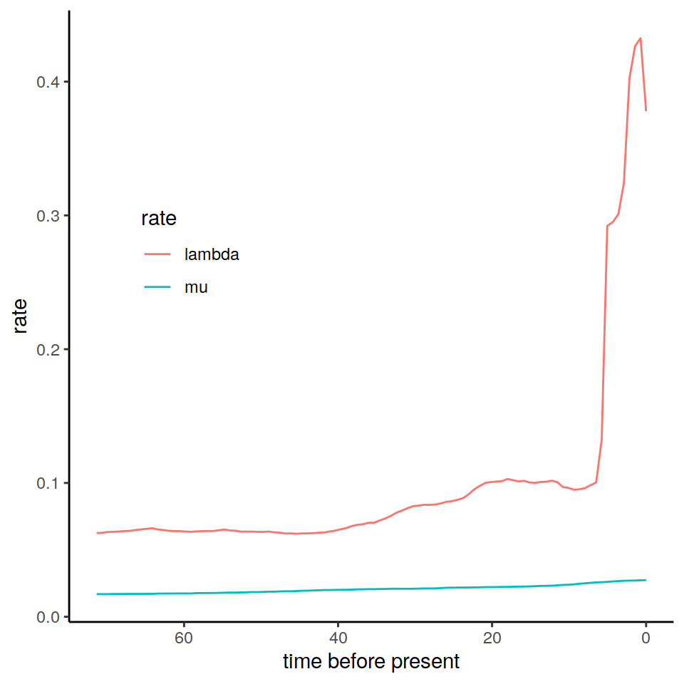
Now let’s have a look at the estimated rate functions
p <- primates_ebd_revbayes %>%
  tidyr::gather("rate", "value", -time) %>%
  ggplot(aes(x = time, y = value, color = rate)) +
  geom_line() +
  theme_classic() +
  scale_x_reverse() +
  theme(legend.position = c(0.2, 0.6)) +
  labs(y = "rate", x = "time before present")
plot(p)
Figure 8.2: The estimated posterior median results from an episodic birth-death model fitted in RevBayes.
The data frame primates_ebd_revbayes is essentially equal to the data frame we get when we call the data("primates_ebd") function in CRABS. We use these estimated rates in our vignette examples, but we note that it is possible to use any kind of rate functions to construct the congruence class.