6 Exploring the congruence class

In theory there are infinitely many speciation and extinction rate functions that are within a congruence class, i.e., all rate functions that have exactly the same likelihood. It is clearly impossible to enumerate all rate functions. Instead of trying to explore literally all rate functions, we will sample from these rate functions instead. This idea is very similar to all sampling based methods. For example, a posterior distribution with a 95% credible interval between 0.01 and 0.02 contains infinitely many values, but we are we comfortable today with simply sampling values proportional to their posterior probability and looking/plotting the distribution.

6.1 Assumptions on rates

There are several plausible assumptions that can be made about diversification rates and how these rates vary.

First, you could make assumptions about the magnitude of rate variation, and specifically what are plausible minimum and maximum rates. Clearly, speciation and extinction rates should not have been smaller than 0, so that could be a safe assumption.

Depending on your study system, you could also assume that rates were never larger than, say, 10 events per lineage per million years. For example, if you would have a speciation rate of 10 per lineage per million years, then you would expect every lineage to speciate on average every 0.1 million years. If there would be no extinction, then this would leave the group with just above 22,000 species after only one million years. So perhaps a rate of 10 could really be seen as an upper bound in systems such as vertebrates and plants. However, you could argue that there is extinction, and we should better restrict the net-diversification rates to be at most 10. We get into some more of these restrictions in another section.

The second assumption is about how rates vary over time. One could argue that if diversification rates were low, say 42 million years ago, then you would assume that the diversification rates were also low 43 million years ago. This would mean that diversification rates are autocorrelated and do not vary completely arbitrarily over time.

In the next subsections, we explore a few different options of rate variation over time in the next sections, which include:

HSMRF (autocorrelated) rates
Exponentially decreasing rates with stochastic variation
Linearly increasing rates with stochastic variation
Episodic constant models (with \(n\) episodes)
Uncorrelated (independent) rates

With the built-in functions sample.basic.models and sample.rates, users have freedom to explore these, and many other forms of rate variation. If these functions are not sufficient, as shown in previous sections, it is easy to customize the sampling to your liking.

6.2 Independent or joint rate sampling

CRABS offers 3 approaches to sample rates:

generate speciation rates, then construct congruent extinction rates;
generate extinction rates, then construct congruent speciation rates;
generate a \(p\)-trajectory, which corresponds to a unique pair of congruent speciation and extinction rates. Independent rate sampling (1 and 2) can be done using sample.basic.models or sample.rates, while joint sampling (3) can be done using sample.basic.models.joint.

The choice between independent and joint rate sampling depends on the assumptions you’re willing to make. Independent sampling allows you to explore specific classes of scenarios for either speciation and extinction rates, while the joint sampling approach offers more flexibility by imposing less constraints on the rates. Andréoletti & Morlon (2023) showed that the joint sampling approach is better able to recover trajectories where the congruence class contains signal for temporal variations both in speciation and extinction rates (which by construction cannot be captured with independent sampling of either rates).

The 3 approaches are presented in more details bellow.

6.3 Sample alternative extinction rates

6.3.1 Temporally autocorrelated

Here, we generate a variety of alternative extinction rates using HSMRF models (Magee et al., 2020). When sampling from models, we get random walks, or temporally autocorrelated, extinction rates, and the HSMRF tends to produce random walks that look like piecewise constant functions. The rates produced here have no overall trend, the median change from past to present is 0. We use the function sample.basic.models to construct these rates, which by default assumes that rates are between 0 and 10, though here we change these boundaries slightly to bound the rates to be between 0 and 1. Our motivation for these values was, that (i) having a maximal expected extinction time per lineage of 1.0 million years seems reasonable from the fossil record, and (ii) we estimated a maximal speciation rate of 0.4, which is clearly smaller than 1.0.

times <- seq(0, max(my_model$time), length.out = 100)
extinction_rate_samples <- function() {
   sample.basic.models( times = times,
                        model="MRF",
                        max.rate=1)
}

samples <- sample.congruence.class(
  my_model,
  num.samples=10,
  rate.type="extinction",
  sample.extinction.rates=extinction_rate_samples)

We can plot the samples using

plot(samples)

Figure 6.1: Rate functions assuming HSMRF-distributed extinction rates

p <- summarize.trends(samples,
                      threshold = 0.02)
plot(p)

Figure 6.2: Congruence class assuming linearly changing extinction rates.

As we can see, the alternative models are not in perfect agreement about the entire history of the rates. Nonetheless, the increases and decrease near the present are preserved, indicating robustness to this form of extinction-rate variation.

6.3.2 Exponentially decreasing

Here, we generate a variety of alternative extinction rates using HSMRF models (Magee et al., 2020) with an exponential trend. We otherwise make the same assumptions as above. To help the rates we simulate fit within 0 and 1, we set the fold change average to be 2 instead of the default 3.

times <- seq(0, max(my_model$time), length.out = 100)
extinction_rate_samples <- function() {
   sample.basic.models( times = times,
                        model="exponential",
                        max.rate=1,
                        fc.mean=2)
}

samples <- sample.congruence.class(
  my_model,
  num.samples=10,
  rate.type="extinction",
  sample.extinction.rates=extinction_rate_samples)

We can plot the samples using

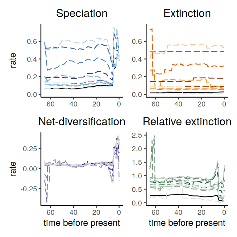
plot(samples)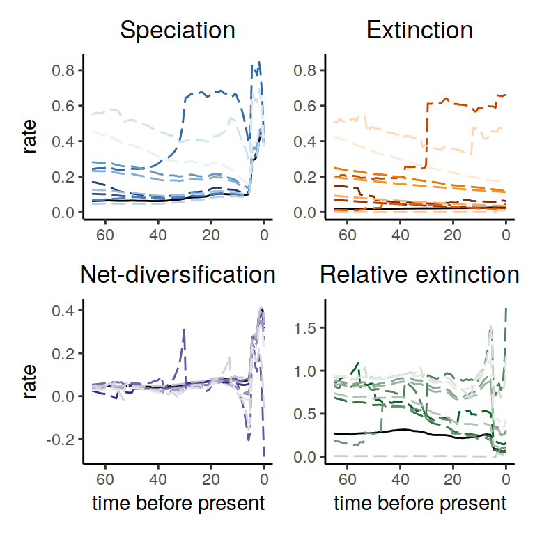

Figure 6.3: Rate functions assuming exponential trends in the extinction rate

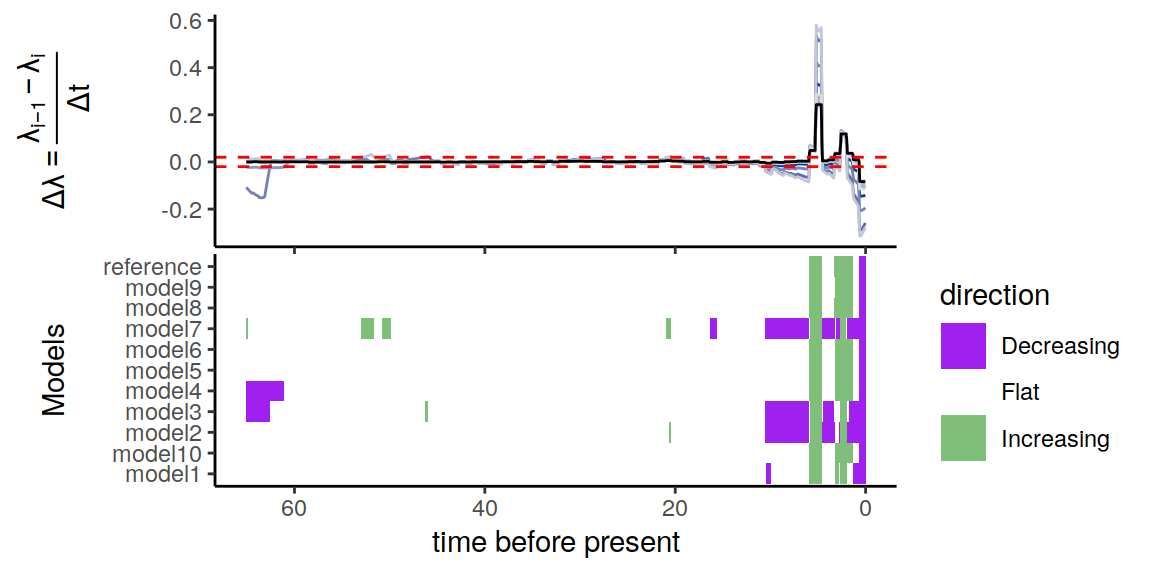
p <- summarize.trends(samples, threshold = 0.02)
plot(p)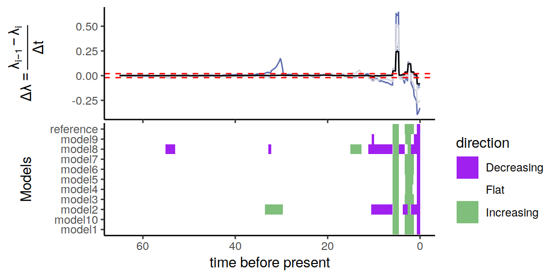

Figure 6.4: Congruence class assuming exponentially changing extinction rates

6.3.3 Linearly increasing

Here, we generate a variety of alternative extinction rates using GMRF models (Magee et al., 2020) with a linear trend. Unlike the exponential section, we here assume that rates have increased, that the increase has been monotonic (there were no decreases, where in the exponential decreases above there were occasional increases), and that the stochastic variability comes from a GMRF. We otherwise make the same assumptions as above.

times <- seq(0, max(my_model$time), length.out = 100)
extinction_rate_samples <- function() {
   sample.basic.models( times = times,
                        direction="increase",
                        model="linear",
                        monotonic=TRUE,
                        MRF.type="GMRF",
                        max.rate=1,
                        fc.mean=2)
}

samples <- sample.congruence.class(
  my_model,
  num.samples=10,
  rate.type="extinction",
  sample.extinction.rates=extinction_rate_samples)

We can plot the samples using

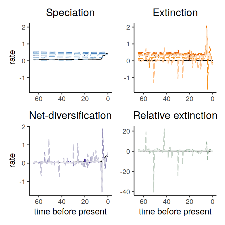
plot(samples)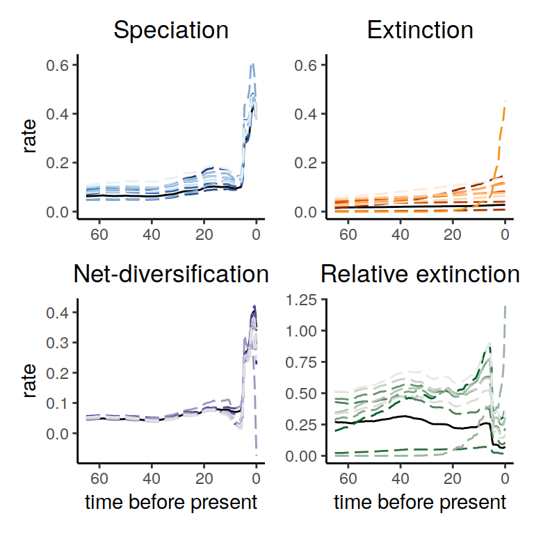

Figure 6.5: Congruence class assuming linearly changing extinction rates.

p <- summarize.trends(samples, threshold = 0.02)
plot(p)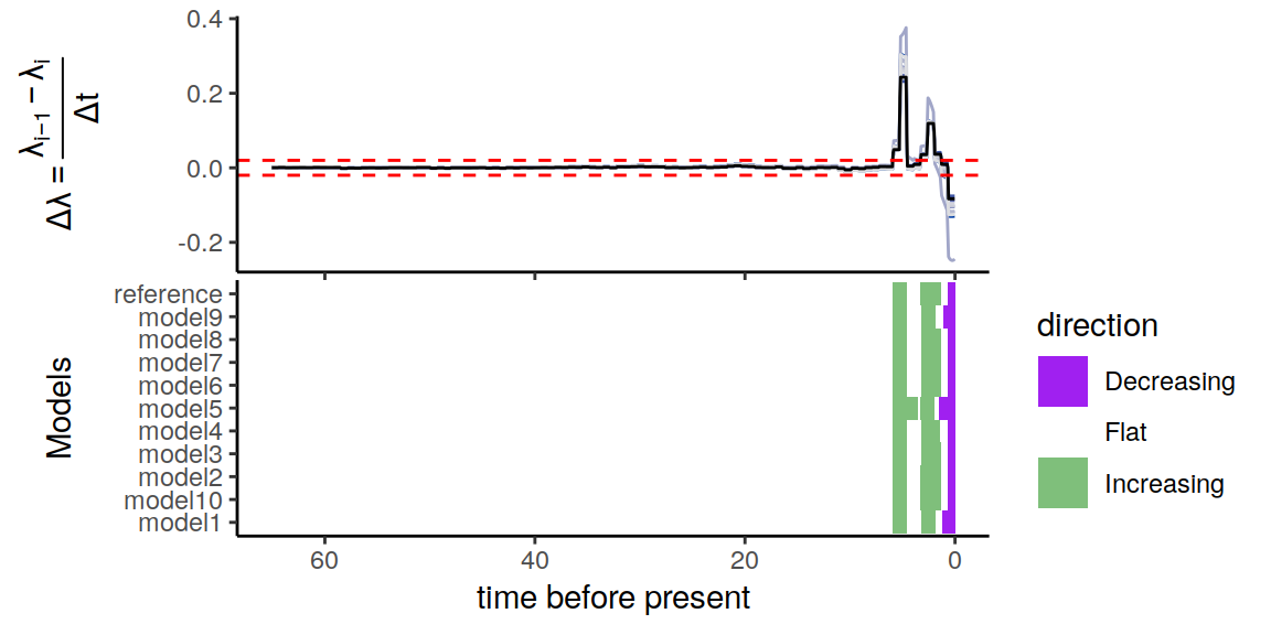

Figure 6.6: Congruence class assuming linearly changing extinction rates.

As we can see, the increases and decrease near the present are preserved, indicating robustness to this form of extinction-rate variation. Compared to the exponential and HSMRF models above, there is even better agreement between the alternative models.

6.3.4 Episodic

Here, we generate a variety of alternative extinction rates without stochastic noise. Without noise (noisy=FALSE), all changes will be in the same direction, here decreases. The model we generate is an episodic model with 5 rates. Here, we consider decreasing rates with larger changes from past to present than the previous section. To help rates stay within the [0,1] bounds we have chosen, we set the rate median at present to be slightly smaller than the default 0.1.

times <- seq(0, max(my_model$time), length.out = 100)
extinction_rate_samples <- function() {
   sample.basic.models( times = times,
                        direction="decrease",
                        model="episodic5",
                        noisy=FALSE,
                        max.rate=1,
                        fc.mean=4,
                        rate0.median=0.05)
}

samples <- sample.congruence.class(
  my_model,
  num.samples=10,
  rate.type="extinction",
  sample.extinction.rates=extinction_rate_samples)

We can plot the samples using

plot(samples)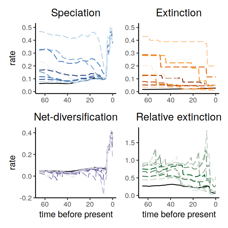

p <- summarize.trends(samples, threshold = 0.02)
plot(p)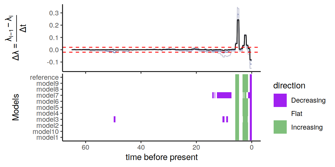

Figure 6.7: Congruence class assuming episodically changing extinction rates.

As we can see, the increases and decrease near the present are preserved, indicating robustness to this form of extinction-rate variation. The agreement between the alternative models is comparable to the linear scenarios above, and higher than for the exponential and HSMRF models.

6.3.5 Uniform independent

The previous functions used sample.basic.models to construct a variety of pre-defined hypotheses. CRABS also implements sample.rates to allow more flexibility in user-defined rate functions (and of course the user is free to define their own functions as well). Here we show this with IID rates. We assume that the extinction rates could have had any value between 0 and 1 (you could easily pick different numbers here). Our motivation for these values was, that (i) having a maximal expected extinction time per lineage of 1.0 million years seems reasonable from the fossil record, and (ii) we estimated a maximal speciation rate of 0.4, which is clearly smaller than 1.0.

We furthermore assume that each extinction rate is independent of the previous time interval. That means that we can model any rate function, even completely crazy zig-zagging functions.

coarse_times <- seq(0, max(my_model$time), length.out = 10)
rsample_extinction <- function(n) runif(n,0,1)
extinction_rate_samples <- function() {
   sample.rates( times = coarse_times,
                 rsample=rsample_extinction,
                 rsample0=NULL,
                 autocorrelated=FALSE)
}

samples <- sample.congruence.class(
  my_model,
  num.samples=10,
  rate.type="extinction",
  sample.extinction.rates=extinction_rate_samples)

We can plot the samples to inspect them visually

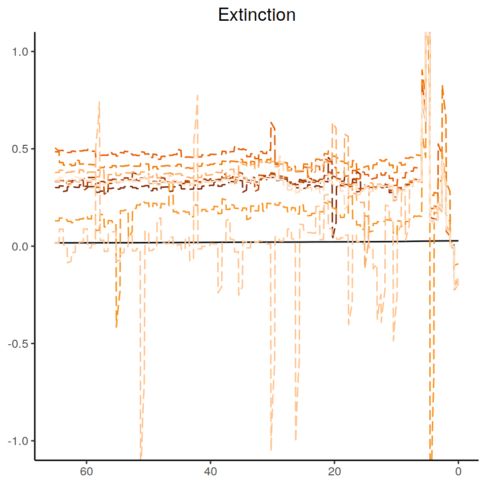
plot(samples)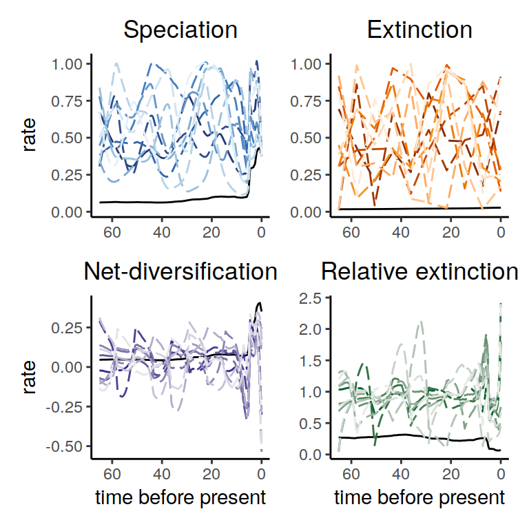

Rate functions for the congruence class with proposed alternative extinction rates whose values are drawn from an independent uniform distribution for each episode.

Figure 6.8: Rate functions for the congruence class with proposed alternative extinction rates whose values are drawn from an independent uniform distribution for each episode.

Next we can plot the directional trends

p <- summarize.trends(samples, threshold = 0.02)
plot(p)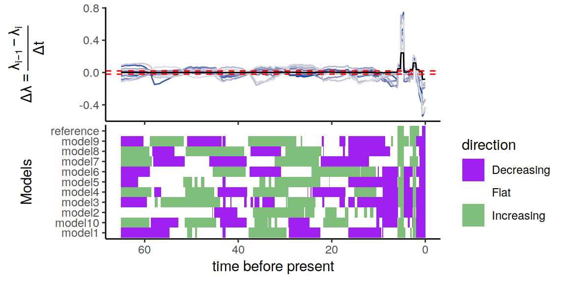

Figure 6.9: Congruence class assuming independent and uniformly distributed extinction rates.

As we can see, the alternative models present many distinct histories of the rates through time. Nonetheless, even in this extreme scenario, the increases and decrease near the present are preserved.

6.3.6 Brownian motion with a trend

It is also possible to specify fully customized rate sampling functions, and use these to sample the congruence class in CRABS. Suppose we thought that the extinction rate was tiny when the clade emerged, but steadily rose in a linear fashion towards the present. Additionally, suppose we allow for some random variation around this linear increase. This can be implemented as a Brownian motion with a trend, as follows.

med_times <- seq(0, max(my_model$time), length.out = 30)

extinction_rate_samples <- function(){
  noise <- cumsum(rnorm(30, mean = 0, sd = 0.03))
  y <- -0.008*med_times + noise + 0.6
  y <- ifelse(y < 0.001, 0.001, y)
  f <- approxfun(med_times, y)
}

For simplicity, we restrict rates that are very small or negative to be a minimum of 0.001 units. As before, we can use CRABS to sample from the congruence class using this form of proposed extinction rates, and plot the rates:

samples <- sample.congruence.class(
  my_model,
  num.samples=15,
  rate.type="extinction",
  sample.extinction.rates=extinction_rate_samples)
plot(samples)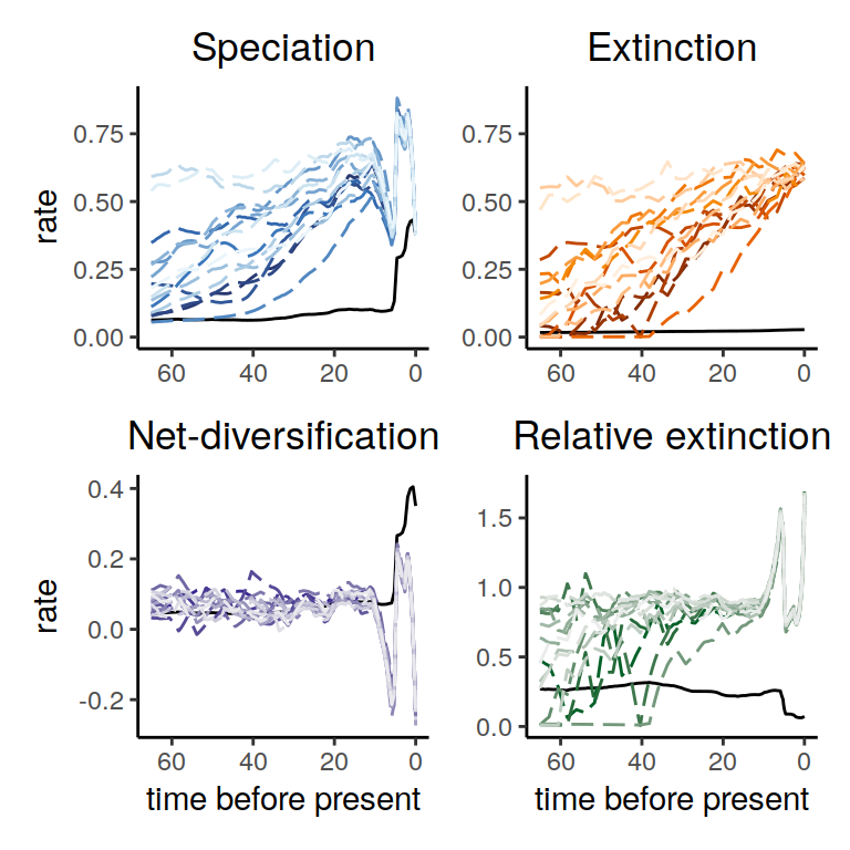

Rate plots for the congruent models that were sampled assuming an extinction rate modeled as a Brownian motion with a linearly increasing trend

Figure 6.10: Rate plots for the congruent models that were sampled assuming an extinction rate modeled as a Brownian motion with a linearly increasing trend

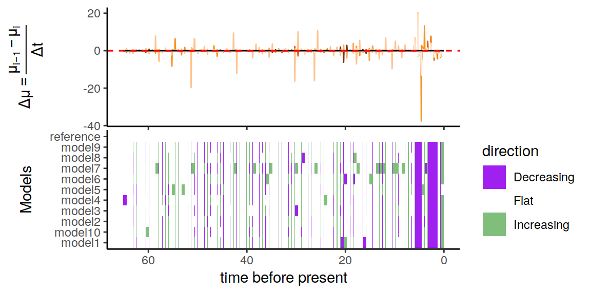
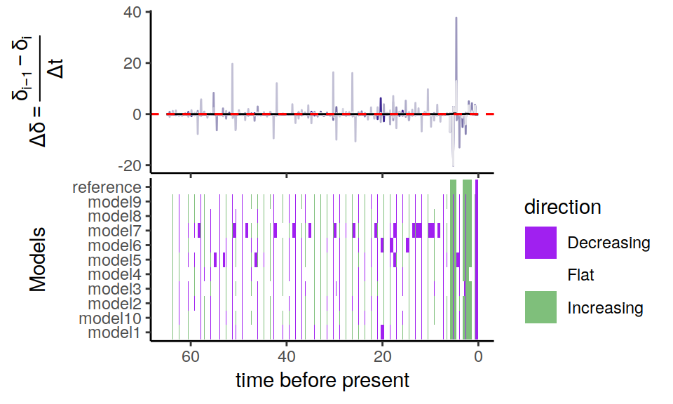
The summary of trends across these models contain quite a bit of variation. However, the three main signals in the primate reference model are all recovered: two increases and one decrease in the recent part of the phylogeny 6.11.

p <- summarize.trends(samples, threshold = 0.02)
plot(p)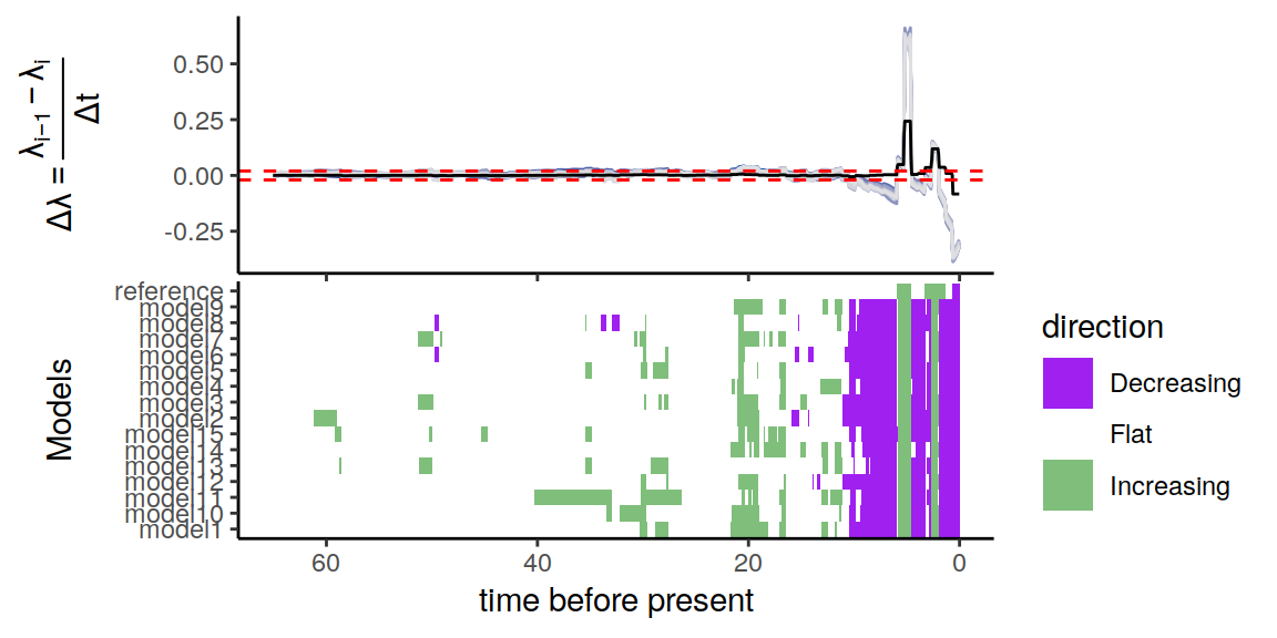

A summary of directional trends through time across the congruent models. The proposed extinction rate is modeled as a Brownian motion with a trend that increases linearly towards the present.

Figure 6.11: A summary of directional trends through time across the congruent models. The proposed extinction rate is modeled as a Brownian motion with a trend that increases linearly towards the present.

6.4 Sample alternative speciation rates

It is also possible to sample alternative speciation rates. Since the congruence class requires a shared \(\lambda_0\) for all models in the congruence class, we must constrain our sampler to always start on the same speciation rate at the present.

6.4.1 Temporally autocorrelated

Here we choose to sample speciation rates according to a horseshoe Markov random field distribution.

times <- seq(0, max(my_model$time), length.out = 100)
speciation_rate_samples <- function() {
   sample.basic.models( times = times,
                        rate0 = my_model$lambda(0.0),
                        model = "MRF",
                        MRF.type = "HSMRF",
                        max.rate = 1.0)
}

Next, we can sample ten models from the congruence class.

samples <- sample.congruence.class(
  my_model,
  num.samples=10,
  rate.type="speciation",
  sample.speciation.rates = speciation_rate_samples)

We can plot the samples using

plot(samples)

Rate functions for the congruence class. The reference model is given in black. The alternative speciation rates are proposed by sampling from a temporally autocorrelated (HSMRF) model.

Figure 6.12: Rate functions for the congruence class. The reference model is given in black. The alternative speciation rates are proposed by sampling from a temporally autocorrelated (HSMRF) model.

Notice that all of our congruent models have a negative extinction rate near the present. This becomes more evident if we plot the extinction rates on its own panel and adjust the axis limits.

p <- plot(samples)[[2]] + 
  coord_cartesian(ylim = c(-1, 1)) +
  xlab("time before present") +
  ylab("rate")
plot(p)

Figure 6.13: Inferred congruent extinction rates, zoomed in for clarity.

The models depicted in 6.13 do not make sense, since rates are only defined on the positive numbers. Similarly to before, we can evaluate the directional changes in the extinction rate

p <- summarize.trends(samples, threshold = 0.02, rate_name = "mu")
plot(p)

Figure 6.14: A summary of directional trends through time across the congruent models.

Notice how the reference model (top row) is flat throughout the entire time span. Yet, when we propose alternative speciation rates, the inferred (extinction) rates depict a pattern of two decreases and one increase in the near present. We can also inspect the directional trends for the net-diversification rate (\(\delta(t) = \lambda(t) - \mu(t)\))

p <- summarize.trends(samples, threshold = 0.02, rate_name = "delta")
plot(p)

Directional trends in the net-diversification rate. The congruence class was constructed using alternative speciation rates, and all congruent models have negative extinction rates.

Figure 6.15: Directional trends in the net-diversification rate. The congruence class was constructed using alternative speciation rates, and all congruent models have negative extinction rates.

6.5 Jointly sample alternative speciation and extinction rates

Here, we simultaneously generate a variety of congruent speciation and extinction rates (Andréoletti & Morlon, 2023). We use the function sample.basic.models.joint to construct these rates. As explained in section 3.3, this function first samples \(p\)-trajectories – controlling the degree to which the signal in the congruence class is driven more by speciation rate variations (\(p=1\)) or extinction rate variations (\(p=0\)) – and then constructs the corresponding speciation and extinction rates.

The procedure for drawing, centering and rescaling a \(p\)-trajectory is explained in Andréoletti & Morlon (2023).

The initial value \(p_0\) is sampled from a Beta distribution. By default, we use \(\beta_1=0.3\) and \(\beta_2=0.3\) to favor starting points near \(p=0\) or \(p=1\). Below we set \(\beta_1=0.5\) and \(\beta_2=0.2\) to place more emphasis on values close to \(p=1\) (constant extinction), ensuring that we properly explore these scenarios. The speciation rate at present is fixed to the reference scenario, while the extinction rate at present is drawn from a log-normal distribution.

6.5.1 Constant joint trajectory

First, we set the scaling factor of the Markov Random Field (mrf.sd.scale) to \(0\), such that we obtain constant \(p\)-trajectories.

joint_rate_samples <- function(){sample.basic.models.joint(
  times = seq(0, max(primates_ebd$time), length.out=300),
  p.delta = my_model$p.delta,
  mrf.sd.scale = 0,
  beta.param = c(0.5,0.2),
  lambda0 = my_model$lambda(0),
  mu0.median = my_model$mu(0))}

samples_primates_CT <- sample.congruence.class(
  my_model,
  num.samples=20,
  rate.type="joint",
  sample.joint.rates=joint_rate_samples)

plot(samples_primates_CT)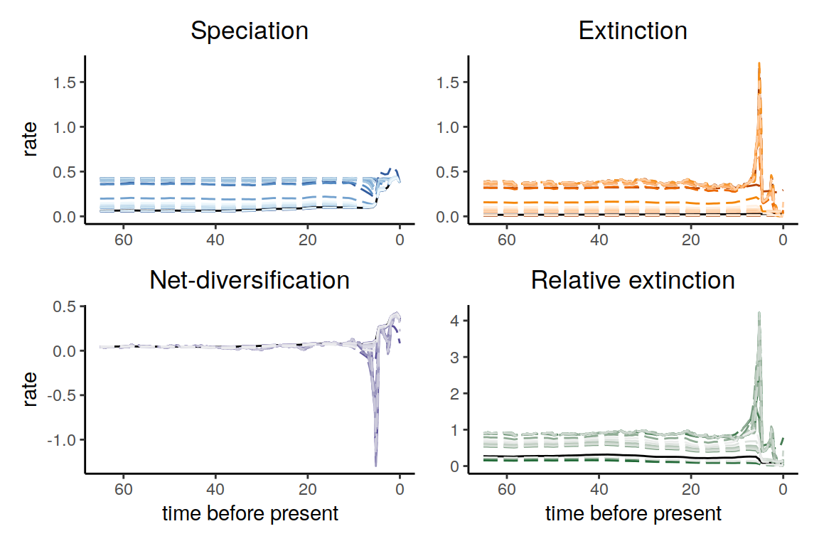

Figure 6.16: Congruent diversification scenarios, jointly sampled with constant p-trajectories.

6.5.2 HSMRF joint trajectory

Then, we revert to the default scaling factor (\(\sigma_{\text{MRF}}=1\)) and use the HSMRF sampler for \(p\)-trajectories.

joint_rate_samples <- function(){sample.basic.models.joint(
  times = seq(0, max(primates_ebd$time), length.out=500),
  #times = my_model$times,
  p.delta = my_model$p.delta,
  MRF.type = "HSMRF",
  beta.param = c(0.5,0.2),
  lambda0 = my_model$lambda(0),
  mu0.median = my_model$mu(0))}

samples_primates_HST <- sample.congruence.class(
  my_model,
  num.samples=20,
  rate.type="joint",
  sample.joint.rates=joint_rate_samples)

plot(samples_primates_HST)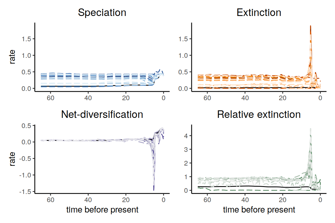

Figure 6.17: Congruent diversification scenarios, jointly sampled with HSMRF p-trajectories.

6.5.3 HSMRF joint trajectory with global regularity filter

Finally, we sample 1000 HSMRF trajectories, with the aim of selecting the smoothest ones (as a proxy for simplicity or parsimony).

joint_rate_samples <- function(){sample.basic.models.joint(
  times = seq(0, max(primates_ebd$time), length.out=500),
  p.delta = my_model$p.delta,
  MRF.type = "HSMRF",
  beta.param = c(0.5,0.2),
  lambda0 = my_model$lambda(0),
  mu0.median = my_model$mu(0))}

samples_FHST <- sample.congruence.class(
  my_model,
  num.samples=1000,
  rate.type="joint",
  sample.joint.rates=joint_rate_samples)

The resulting trajectories are filtered according to a given regularity penalty (by default a \(\mathcal{L}_1\) norm) and several thresholds.

full.plot.regularity.thresholds(samples_FHST, filtering_fractions = c(0.05, 0.2, 0.9))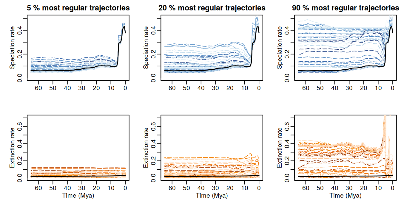

Congruent diversification scenarios, jointly sampled with HSMRF p-trajectories and selected based on their regularity, for decreasingly stringent thersholds.

Figure 6.18: Congruent diversification scenarios, jointly sampled with HSMRF p-trajectories and selected based on their regularity, for decreasingly stringent thersholds.

Other penalties can be specified, among the following (“L1”, “L2” and “L1_derivative”):

The \(\mathcal{L}_1\) norm on all the step-wise variations in both speciation \((\lambda_i)\) and extinction rates \((\mu_i)\), for \(i \in [\![0;N]\!]\), where \(N\) is the number of time steps : \[\mathcal{L}_1 = \sum_{i=1}^N \left[abs(\lambda_i-\lambda_{i-1})+abs(\mu_i-\mu_{i-1})\right]\] The \(\mathcal{L}_1\) norm sums the absolute differences between consecutive speciation and extinction rates. Rate trajectories with low \(\mathcal{L}_1\) norms tend to have few and small rate variations.
The \(\mathcal{L}_2\) norm on step-wise variations: \[\mathcal{L}_2 = \sqrt{\sum_{i=1}^N \left[(\lambda_i-\lambda_{i-1})^2+(\mu_i-\mu_{i-1})^2\right]}\] The \(\mathcal{L}_2\) norm, also known as the Euclidean norm, squares step-wise differences before summing and taking the square root. This has the effect of penalizing larger jumps more severely than smaller ones.
The second-order \(\mathcal{L}_1\) norm on derivative shifts in both speciation and extinction rates: \[\mathcal{L}_1' = \sum_{i=2}^N \left[abs(\lambda_i-2\lambda_{i-1}+\lambda_{i-2})+abs(\mu_i-2\mu_{i-1}+\mu_{i-2})\right]\] The second-order \(\mathcal{L}_1\) norm (\(\mathcal{L}_1'\)) focuses on the change in the rate of change, effectively measuring the volatility in the trajectory. This offers an additional layer of smoothness by considering how rate changes are themselves changing.