How not to measure the dimensionality of treespace

As you can perhaps tell from the title, this is a post about failure. Awhile ago, I got what I thought was a clever idea¹. And I was so sure of myself I jumped straight to making a repo for the code that would assuredly lead to a brilliant manuscript². I’m leaving it up as a testament to my failure, but since the problem still bugs me, I’m writing this up.

The scientific question

A question that comes up in phylogenetic contexts a lot is “do these two loci share a phylogeny?” In particular, I’m talking about cases where we’re interested in underlying differences in topology, and not simply branch lengths³. The last time this question came up for me, I was trying to identify recombination breakpoints in some viral genomes. But this question can also come up if we’re feeling lazy and don’t really want to use species tree methods and hope we can just concatenate things. Or even if we’ve given up and know we need the multispecies coalescent but want to reduce the number of gene trees involved.

From a statistical perspective, we can frame this as a hypothesis test, or as model selection. For simplicity’s sake, let’s consider only two loci, so our models are that there is one tree, or that there are two trees. If we want to do hypothesis testing, we need some (asymptotic) distribution of a test statistic, like in a likelihood ratio test (LRT), where (twice) the difference in maximized log-likelihoods between the models follows (approximately, asymptotically) a chi-squared distribution. (Or we need to undertake am expensive brute-force simulation-based approach⁴.) If we want to do model selection, and we don’t want to wait on marginal likelihoods⁵, we might like to do something like AIC or BIC, to penalize the two-tree model for complexity. Either way, we need to know how much more complex the two-tree model is. That is, how many more parameters does it have? The easy part: it has twice as many branches. The hard part: it has twice as many trees.

My not-so-clever methodology

In brief, my notion to address this question was to swap around input and output in a LRT. Roughly speaking, a LRT takes in as input the degrees of freedom (the difference in the number of free parameters between the more complex and the nested simpler model), an observed difference in log-likelihoods between two models, and outputs a probabilistic judgement on whether the more complex model is justifiably better. It does this via the asymptotic approximation that the distribution of the LRT statistic is chi-squared. What I had in mind was to feed in many observed differences in log-likelihood, a known judgement on whether the complex model is justifiably better (it would not be), and output the degrees of freedom.

What is Normal, anyways?

If that doesn’t make sense⁶, let’s try an example. And for the moment, let’s stick with Normal distributions⁷. Imagine that I tell you I will simulate independently $m$ times from the following experiment. I draw $kn$ observations, where $n$ is large, of a Normal($\mu$, $\sigma^2$) distribution. Then I fit two models, and give you their likelihoods. The simpler (null) model is that all $kn$ draws come from the same Normal, whose mean and variance I estimate. The more complex model is, for some $k$, that there are $k$ sets of $n$ draws, each from their own Normal distribution whose mean and variance I estimate.

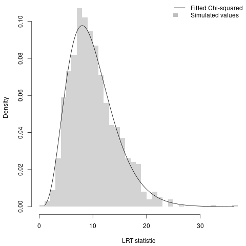
You might choose to record, per experiment, twice the difference in log-likelihoods of the two models. Then, the $m$ values are independent draws from a distribution which is asymptotically Chi-squared, with $2(k - 1)$ degrees of freedom (where the 2 is because you know that each component comes with a mean and a variance to estimate). This means that, in theory, you can fit $k$ to the $m$ LRT statistics and tell me what it is.

Now, the question, does it work? The answer would seem to be yes. When I simulate 1000 times with $k = 6$, the best-fitting Chi-squared distribution has 10 degrees of freedom, which is the right answer.

The results for trees

My plan for trees was pretty similar. For each experiment, at a given tree length and number of tips, I would simulate one true tree. I would then simulate an alignment with $2n$ sites in it, and fit two models with maximum likelihood, a one-tree model and a two-tree model. To keep things simple, I’d use Jukes-Cantor so that the difference in free parameter count between the models would be the tree topology and the number of branches.

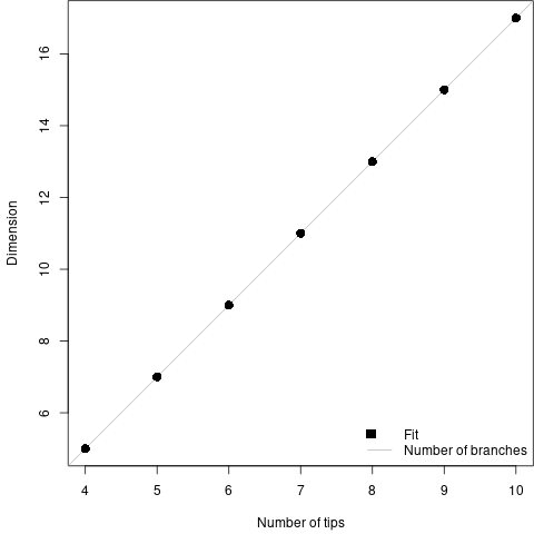
I decided to do this for 4 through 10 tip trees, because IQ-TREE can infer trees that size nearly instantaneously so 200 replicates at each tree size for a few tree lengths would be feasible before I tried to scale up.

However, when I summarized these simulations, to my surprise I found that the degrees of freedom was simply the number of branches in the tree. This meant that I was inferring that the number of free parameters a tree was worth was… 0. Because all the free parameters were going into the branch lengths on the second tree.

What went wrong?

So, why did this go off the rails?

The LRT is an asymptotic result, and as such I chose to simulate large alignments of 100,000 sites. For the shortest simulated tree length (0.25) for the largest tree (10 tips, 17 branches) the average branch has 1470.6 substitutions on it. That’s probably large enough for the asymptotics, but unfortunately it’s also a guarantee that we get the right tree topology every time⁸. In other words, the effect of the tree topology isn’t showing up in our simulations because, in the region we’re simulating, there is no effect of the tree topology.

Really, then, the problem is that I tried to use an asymptotic tool to answer a non-asymptotic question. The effect of phylogenetic uncertainty lives in a world where we don’t have an effectively infinite amount of data about the topology. Given how skeptical I often am about asymptotic results, I feel like I should have seen this coming in advance. Alas.

1. This is always a warning sign. Trying to be clever produces bimodal outcomes and the bigger mode is decidedly “well that wasn’t such a good idea, now, was it?” ↩

2. This is why we have sandbox repos where we FA before inevitably FOing. ↩

3. This is just a question of continuous model parameters, so it fits in the usual statistical toolkit just fine. ↩

4. For example, fit the one- and two-tree models to real data, compute the difference in likelihood. Then, to get the null distribution, simulate a few hundred alignments under the one-tree model. Fit both one- and two-tree models to each, record the difference in likelihood. Easy, but slow. ↩

5. Though perhaps this is a good use-case for one of our 19 dubious approaches for fast approximate marginal likelihoods? ↩

6. And it didn’t when I tried to explain it to a much smarter colleague, so perhaps again I should have known I was destined for trouble. ↩

7. As always, the statistician’s crutch. ↩

8. At least here where we’re not simulating funky non-neutral substitution models. ↩